Vehicle Signal Burst Analysis

In some cars of BMW’s test fleet, an odd issue occurred: Under certain circumstances the cars’ various systems would send too many messages over the internal communication bus, leading to low priority messages being delayed for long times.

Given several log files, our task was to investigate the cause of this issue by finding features that correlate with the observed signal bursts, which required us to build interpretable models for anomaly detection on time-series data. During the project, we presented and discussed our progress regularly within the TUM Large Scale Machine Learning Lab and showcased our findings during a final poster session at TUM.

Project Overview

• Duration: April to August 2019 (5 months)
• Team: Two other M.Sc. Data Science/Robotics students and me
• My Responsibilities: Data cleaning and preparation; GBDT implementation, training, and interpretation

Data Preparation

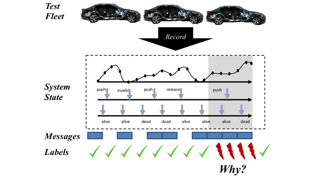
The data we received from BMW was in the form of multiple log files, which contained one entry with corresponding timestamp per internal message sent or per state change in the system. Many of the rows contained nulls, NaNs, and other invalid entries, so a lot of time had to be spent on data cleaning before we could start our analysis.

Furthermore, we encoded all categorical variables and created several hundred additional aggregate variables, such as the latest logged message for each state or the amount of time that a given state had not been changed.

In one of the log files, we also had timestamps for all signal bursts that occurred. Based on this information, we added labels to each sample: if the time to a burst was less than a fixed threshold, we labeled it as burst, otherwise we labeled it as no burst. This allowed us to later train classification models on the data.

In the end, our dataset consisted of roughly 6 Million samples with around 1700 variables, for a total of ~10 Billion values. The sheer size of this dataset was part of the challenge.

Metrics

Since only ~0.5% of our data was labeled as burst, we were dealing with a highly imbalanced classification problem and had to find suitable metrics to measure the performance of our models in a meaningful way. Thus, we tracked several metrics, such as the fraction of bursts found, precision, recall, F1 score, and balanced accuracy.

In the end, we mostly used a combination of balanced accuracy and F1 score for model selection and used balanced accuracy for all quantitative evaluations.

Anomaly Detection with LSTMs

Since we were dealing with time-series data, our first idea was to model the problem using LSTMs (check Colah’s blog for a good LSTM explanation). We built a custom architecture in PyTorch, which first projects the data into a lower-dimensional space based on Wide & Deep Networks, then encodes the embedding into a latent representation, and finally classifies using a fully-connected output layer with weighted BCE loss.

We also experimented with other LSTM-based research papers for anomaly detection but were unable to achieve better results than with our “basic” model. As always, deeper and more complex is not always better, even if it’s tempting.

In the end, we managed to predict bursts reliably and achieved balanced accuracy scores of 0.76 on validation and 0.79 on test.

Gradient Boosting Decision Trees (GBDT)

With LSTMs, we were able to predict quite accurately when a burst was going to occur. But even more important was to find out why the bursts happened. Since LSTMs are notoriously hard to make sense of, we turned to more interpretable approaches from classical machine learning, namely, gradient boosting decision trees (GBDT).

As the name suggests, GBDT is gradient boosting (GB) applied to decision trees (DT). Decision trees are one of the simplest machine learning techniques where we iteratively build a tree of if-else decisions by splitting the data according to the most descriptive feature at each step. By doing so, we effectively separate our data into different groups. To classify unseen data, we then find the corresponding group according to our if-else decision rules and choose the majority label of the group as our prediction.

Gradient boosting is a technique that iteratively combines weak individual models to form a single powerful predictor. How that works is very simple, we start with the best constant model (in classification this is the mode of the labels), then we train one weak model on the cases where the constant model failed, followed by a second model minimizing the error of the first model, and so on until the whole training data is classified correctly. During inference, we then average the predictions of all the models. Since this would overfit really hard, we either prune the final model or just stop adding new models once the validation performance starts decreasing.

TL;DR: GBDT means simply training a bunch of decision trees in a smart way and averaging their results. Now, why is GBDT cool?

1. GBDT is one of the most powerful methods of “classical” machine learning and even outperforms neural networks on many tasks involving structured data (which is why it’s very popular in Kaggle competitions and the like).
2. At the same time, GBDT is just a bunch of trees, which in turn are just a bunch of if-else statements, so we understand very well what is going on.

To implement our GBDTs, we used CatBoost, because it has great visualization features and comes with out-of-the-box multi-GPU support.

During training, we experimented with several versions of our dataset with different aggregate features and also carefully tuned all GBDT hyperparameters manually, thereby training several hundred models in the end.

To further push the limits, we even created an ensemble of our best models, which managed to achieve balanced accuracy scores of 0.89 on validation and 0.76 on test, which is very similar to the LSTM we used before.

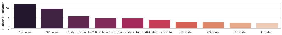
The best individual GBDT achieved a test score of 0.74. Using CatBoost’s feature importance visualization, we were then able to find which of our features had the highest correlation with the occurrence of bursts:

Furthermore, we used the best individual decision tree of the GBDT to extract explicit decision rules that explain under which circumstances bursts occur:

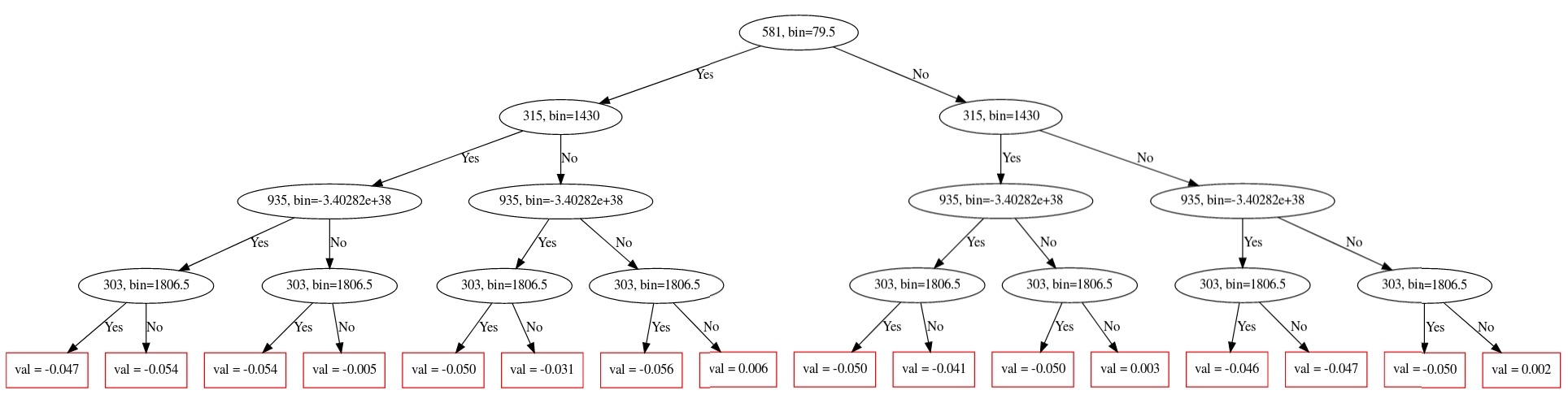
This tree alone also achieved a test score of 0.68, so the rules we extracted should be meaningful.

Result

According to our contact at BMW, the features we identified were coming from a vehicle part that they had already assumed to be a potential cause of the problem. Hopefully, our findings allowed BMW to further narrow down and ultimately fix the issue.

Our supervisors at the lab course were also pleased with the result and graded our project as 1.0.

Takeaways

• When analyzing time-series data, you can incorporate the temporal component either directly into the model (e.g. with recurrent architectures in LSTMs) or into the dataset itself by creating aggregate features. The former is usually slow to train, the latter makes your dataset size blow up. Choose whichever is the lesser of the two evils in your situation.
• Deep learning is very powerful, but sometimes simpler approaches can already do the job well enough while being far easier to train and interpret. “Start simple” also applies to the general model family.
• Choose your performance metrics carefully and define them as early as possible. Then find the best model on your metric. Having this order is a kind of test-driven model development that ensures your results are unbiased.