Paired and Unpaired 2D-to-3D Generation

Generating realistic 3D objects from 2D images is a hot research topic that will form the basis of many exciting AR/VR products of the future. However, the task is fundamentally underconstrained since a given image could have been produced by a multitude of plausible 3D representations.

For our final project in the TUM Advanced Deep Learning for Computer Vision (ADL4CV) class, we experimented with a synthetic dataset of furniture, trying to reconstruct the given 3D models from single-view renderings. We built models for both the paired setting, where the training data consists of object-rendering pairs, and for the unpaired setting, where merely unordered sets of samples of each domain are available.

Project Overview

• Duration: April to August 2019 (5 months)
• Team: Another M.Sc. Informatics student and me
• My Responsibilities: Keras model development

Dataset

We used the Shapenet dataset for all our experiments. However, we simplified it by only using a subset (chairs/tables mainly), and we also removed the texture and used grayscale renderings only.

Additionally, we made several improvements to the dataset and re-rendered it in Blender:

• In original Shapenet, the positions of all voxels are fixed, but the positions of renderings are not. Thus, we rendered all objects from fixed viewpoints such that renderings and voxels are correctly aligned.
• In original Shapenet renderings, very thin parts of the 3D models are often not rendered. We rendered the models more exactly such that also thin parts were included correctly.

Furthermore, we implemented a sophisticated parallelized Tensorflow data pipeline that can load our dataset efficiently, and augment it by rotating 3D voxels on the fly to match given renderings.

Development Environment

Initially, we used Google Colab to train our models. The nice thing about Colab is that you can get free access to a strong GPU, which is absolutely necessary to train GANs. However, the drawback is that your session automatically times out after a fixed amount of time upon which all data is wiped. Thus, you need to do the setup (get code and data onto Colab, install packages, …) every day again and again.

To avoid repeating the data upload (which can take really long), we converted our dataset to TFRecords, uploaded it to our Google Drive, and then mounted Drive in Colab and streamed the data directly from Drive.

In the end, we still decided to switch to a proper Google Cloud instance. There, you can have persistent storage that can easily be loaded into your virtual instance. The big drawback of GCP is that it costs a lot of money if you need a GPU, but it saved us a lot of time, so it was worth it.

Paired Generation

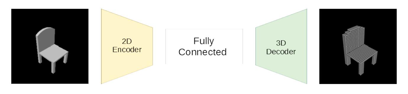
For paired generation, we used a simple encoder-decoder architecture, as shown below.

As loss function, we used a custom voxel-wise weighted BCE loss. Since only ~3% of our voxels were occupied, this was a crucial design choice, as the model would have otherwise been strongly biased towards predicting “not occupied” for a given square.

In case you’re wondering why we didn’t use GANs: it’s because the main advantage of GANs is the high fidelity (i.e., realistic image/output quality), but if your ground truth data only has size 32³ fidelity is not an issue. A simple L1 loss can get the job done too, and it’s much easier to train.

Rule #1 of Deep Learning: always start simple and only use complex stuff if absolutely necessary.

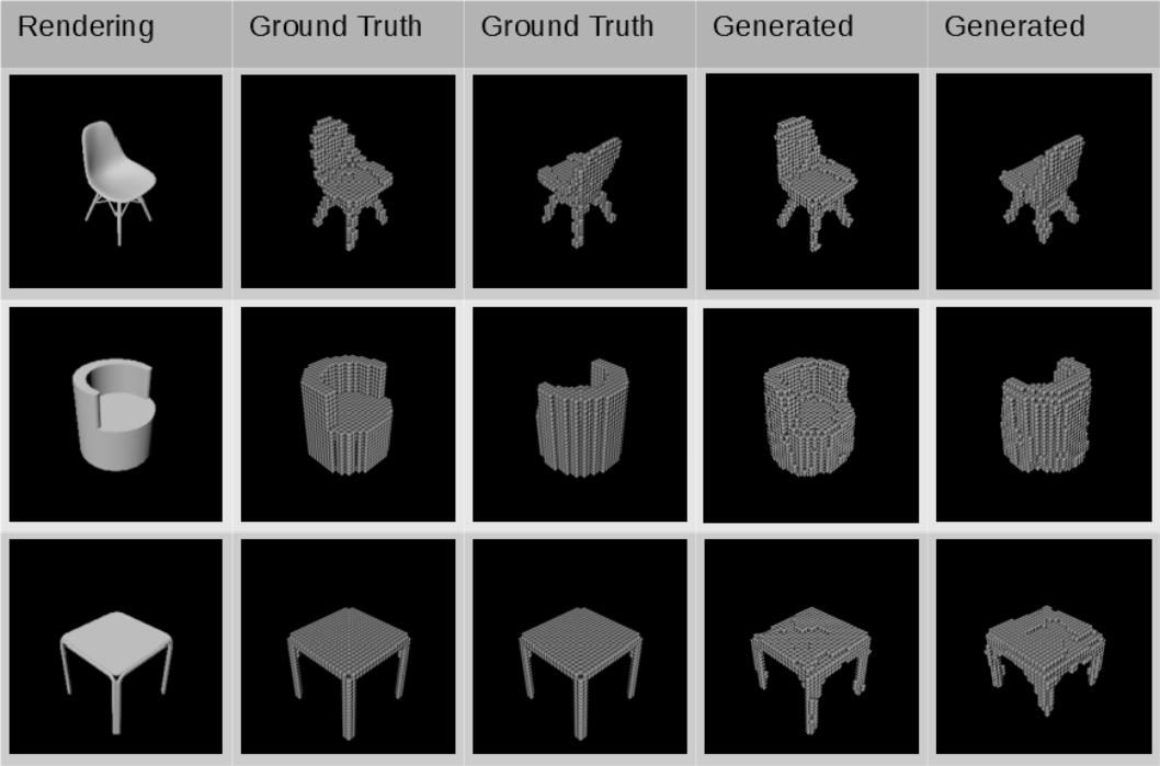
Together with our data fixes, this already allowed us to achieve great validation results as shown below. Note that the model was only trained on chairs, but even managed to generate tables fairly well, which means it also generalizes to some extent.

Unpaired Generation

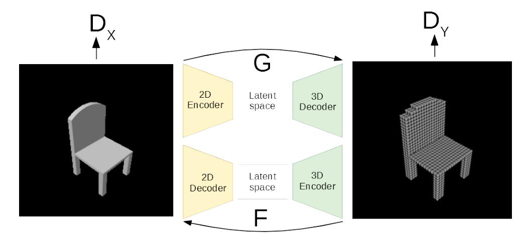
After achieving satisfying performance in paired generation, we decided to relax our assumptions and experiment with unpaired data. What is the difference? Well, in the paired setting, we know how the correct 3D model of a 2D scan looks like, so we can simply constrain the model to produce similar outputs. In the unpaired setting, such information is not available. All we have is a set of unordered 2D scans, and a set of unordered 3D models, i.e., we can give the model examples of each domain but it has to figure out on its own how a sample from one domain should look like when translated to the other.

The most popular model for unpaired image translation is CycleGAN, where two GAN models (one for each translation direction) are trained jointly. See the teaser image for a visualization. Since the original CycleGAN implementation was only available in PyTorch, we reimplemented it in Keras, so we could use it with our existing Tensorflow data pipeline.

When we trained the CycleGAN model, we found it to be very unstable. Initially, there were several hard-to-find bugs that caused the generations to be complete garbage. To find the issues, we broke up the CycleGAN into parts that we tested separately, i.e.:

• Can the discriminators be used for image/voxel classification?
• Can the encoders of the generators be used for classification?
• Can the generators learn with an L1 reconstruction loss?
• Can the two GANs learn unconditional distributions on their own?

After lengthy debugging and several stability improvements with WGAN-GP, Spectral Normalization, and other techniques, we managed to generate outputs that at least somewhat resembled what we wanted. Some examples of input renderings together with corresponding generations are shown below. The model was trained on tables only. 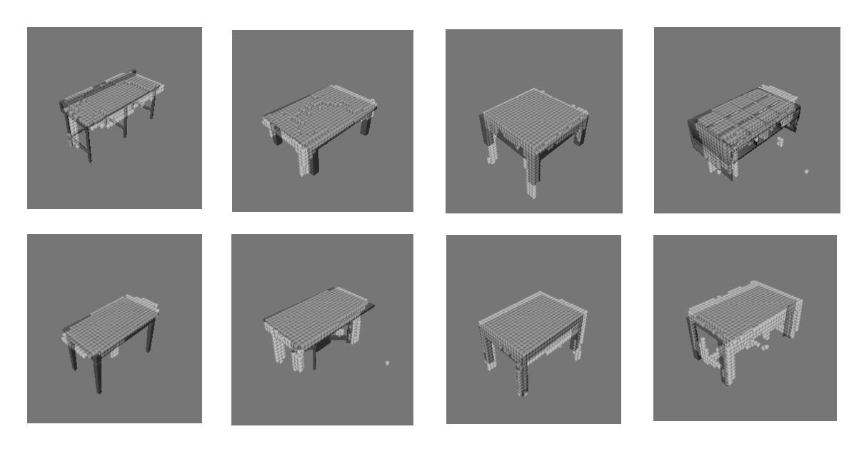As we see, the generations resemble the input, but they are far from perfect. We believe this is a fundamental issue of the model we used since the cycle-consistency loss of CycleGAN assumes a bijectivity between the two domains. If your problem is underconstrained, like 2D-to-3D generation, CycleGAN will, therefore, almost certainly not work well without further modifications.

Pretraining Autoencoders for CycleGAN

To simplify the unpaired learning problem, we also experimented with a pretraining technique we came up with. The basic idea is that you split the two CycleGAN generators into their encoders and decoders, then combine the encoder of one GAN with the decoder of the other and jointly pretrain the two parts as an Autoencoder. I.e., we took the 2D encoder of the 2D-to-3D generator, combined it with the 2D decoder of the 3D-to-2D generator, and trained them jointly to reconstruct 2D images. Then we did the same for the 3D encoder and decoder reconstructing 3D objects, and then used the learned weights as initialization for our CycleGAN.

Qualitatively, we found this technique to improve GAN stability, but we didn’t have time to conduct proper quantitative ablations in the end.

Result

Overall, we implemented a lot of stuff for this project and highly exceeded the expectations of the course. Implementing and training a GAN from scratch is no easy feat, and we additionally built a very strong paired model, rendered our own data, and wrote a complex data pipeline.

As a result, we received almost full points on the project. Since I also did well in the exam, I was one of the only students that achieved grade 1.0 in the end.

Takeaways

• Training GANs is hard. If you can, start with an existing implementation like pix2pix, CycleGAN, etc., and use their hyperparameters. Otherwise, you’ll be in for a world of pain.
• For GANs, as for any other ML model, always start with the most simple architecture and increase complexity as you go. If things don’t work, break your model down into smaller components and debug those separately.
• Before you use an existing ML model, read the paper carefully and make sure you understand for which problems the model is well suited. In our example, it could have been clear from the get-go that CycleGAN would not perform too well since it assumes bijectivity between domains, which is not given in 2D-to-3D generation.
• Good data is key. Sometimes you can spend hundreds of hours tuning your model to get a few more percent of performance, while much more significant improvements could be achieved simply by fixing obvious data problems.